Johannes Haupt remerge.io
Predicting conditional mean and variance
Train a neural network to predict the distribution or uncertainty of a continous outcome, like the win rate distribution in auctions.
Context
In most applications, we build models to predict the expected outcome given some inputs. But for many decisions we aim for a satisfying outcome that minimizes our own effort, cost or risk. How? In my case, I want to win online auctions – and win at a price where I maximize my net value even if that means loosing a few acutions.
For that, I predict the win rate of placing any bid in an auction. If I bid 10 euros, maybe the chance of me winning is 10%. If I bid 20 euros, maybe it increases to 80%. And I’ll place my bid accordingly. In my case, I know the clearing price of previous auctions, so I can predict the average clearing price. Let’s say that’s 15 euros.
Now I could always bid 16 euros, but life is rarely that simple. Clearing prices vary and sometimes the same item goes for 13, other times for 17 euros. If I knew what the spread of clearing prices was for each item, I could try to lowball on items that sometimes sell for much less than their average price. Then again, for items that always sell at market price, I’d rather stick with the average.
From predicting conditional mean to conditional variance
So what’s a conditional mean estimate? That’s easist to see for decision trees: We split the data by some features and then calculate the mean of the outcome in each leaf. So for each leaf, we predict the mean conditional on the feature splits – the conditional mean.
Now we calculate also the variance of the outcome of the training data in each leaf, that’s the conditional variance. If that sounds magical, more fun with forests is in [Athey, S., Tibshirani, J., & Wager, S. (2019). Generalized random forests. The Annals of Statistics, 47(2), Article 2]. In practice, we could take predict the histogram in the leaf or plug the mean and variance into a Gaussian distribution, for example.
Loss function for Gaussian outcomes with variance
If we want to use a neural network, then we’ll need a loss function though. The mean-squared error won’t do, because it only considers the conditional mean prediction. But it gives a good starting point, because it can be derived from this model description:
\[y_i \sim \mathcal{N}(\mu = f(X_i), \sigma^2)\]We model the observed outcomes as random draws from a Normal distribution. The mean of that Normal distribution depends on some input features $X$, the conditional mean, and the outcomes don’t match that exactly because there is some random noise described by the variance $\sigma^2$.
When training a neural network for regression, we optimize the neg. log-likelihood of that model. Don’t believe me? Start with the likelihood of the data (that’s the multiplication) and each data point’s likelihood is the observed outcome $y_i$ and the prediction of the model $\mu_i = f(W,X)$
\[L(y | W,X) = \prod_{i=1}^n \frac{1}{\sqrt{2\pi\sigma^2}}\exp\Bigg(-\frac{(y_i-\mu_i)^2}{2\sigma^2}\Bigg)\]Take the log
\[\ln L( y | W,X) = -\frac{n}{2}\ln(2\pi\sigma^2) - \sum_{i=1}^n \frac{(y_i-\mu_i)^2}{2\sigma^2}\]Now, if we assume $\sigma^2$ is the same for any input, we can pull that out, too, for
\[\ln L( y | W,X) = -\frac{n}{2}\ln(2\pi\sigma^2) - \frac{1}{2\sigma^2}\sum_{i=1}^n (y_i-\mu_i)^2\]We minimize the negative log likelihood and the constant term isn’t relevant for optimization, so that’s just the ol’ MSE.
\[\text{argmin}_{W} \sum_{i=1}^n (y_i-\mu_i)^2\]In our case, we don’t assume that the variance is the same for all inputs. We think it’s different and we want to predict it with our model! With that assumption, we can’t pull the $\sigma^2$ out and ignore it because it’s a constant, so instead we’re left with
\[\text{argmin}_{W} \sum_{i=1}^n \ln(\sigma_i) + \frac{(y_i-\mu_i)^2}{2 \sigma_i^2}\]Andt that’s it, that’s the loss function for our neural network.
Implementation
import numpy as np
import scipy as sp
import matplotlib.pyplot as plt
import tensorflow as tf
from tensorflow import keras
from tensorflow.keras import layers, regularizers
Loss function definition
Tensorflow doesn’t support multiple outputs that are used in the same loss function very well. So be aware that the neural network will output a single output $y_{pred}$, which is a array of $[\text{batch size}, 2]$, where the first column is the mean and the second column is the predicted variance $\sigma^2$
# Define custom loss function for mean squared error just for comparison
def mse_loss(y_true, y_pred):
    return tf.reduce_mean(tf.square(y_true - y_pred))

# Define a custom loss function for a Gaussian output and varying variance
def gaussian_loss(y_true, y_pred):
    # Make sure that the shapes match
    y_true = tf.reshape(y_true, (-1,1))
    mu_pred = y_pred[:, 0:1] # mean prediction
    sigma_pred = y_pred[:, 1:2] # variance prediction

    # Loss function from above
    loss = (
        tf.square(y_true - mu_pred) / (2*(tf.square(sigma_pred)))
    ) +tf.math.log(sigma_pred)

    return tf.reduce_mean(loss)
Example data
As an example, I’ll stick with a simple scenario where we have lots of auctions. The auctions are for one of three products that have different price levels.
- The auctions are also held on three different market places $x_1$, maybe three different websites.
- Depending on the website $x_2$, the clearing price tends to be exactly the market value of the item or it can vary a lot.
- For simplicity, the spread only varies with the market place and the mean only with the item
import numpy as np
import pandas as pd

# set random seed
rand_gen = np.random.default_rng(seed=42)

# 3 products
x1 = rand_gen.choice([0,1,2], size=100000)

# 3 market places
x2 = rand_gen.choice([0,1,2], size=100000)

# set the mean and spread of y for each level of x1
mean_dict = {0: 40., 1: 60., 2: 80.}
std_dict = {0: 1., 1: 10., 2: 5.}

# simulate y, the clearing price
y = np.zeros(100000)


# calculate y for each observation
for i in range(100000):
    y[i] = np.random.normal(loc=mean_dict[x1[i]], scale=std_dict[x2[i]])
I one-hot encode the inputs and drop the first level for each, so we interpret our neural net easily as a linear regression model.
# create a data frame with x1, x2, and y
x1_ohe = np.eye(3)[x1]
x2_ohe = np.eye(3)[x2]
X = pd.DataFrame(np.concatenate([x1_ohe[:,1:], x2_ohe[:,1:]], axis=1))

print(X[:5], "\n\n",y[:5])
     0    1    2    3
0  0.0  0.0  0.0  1.0
1  0.0  1.0  0.0  1.0
2  1.0  0.0  1.0  0.0
3  1.0  0.0  1.0  0.0
4  1.0  0.0  0.0  0.0

 [35.10754029 89.04576279 71.67048054 64.10832465 59.16487619]
np.vstack([x1,x2])
array([[0, 2, 1, ..., 1, 0, 2],
       [2, 2, 1, ..., 0, 2, 2]])
data = pd.concat([
    pd.DataFrame(np.vstack([x1,x2]).transpose(), columns=["floor_price","partner"]),
    pd.DataFrame({"y":y})
], axis=1
)
To make it easier to check model training, let’s see what loss a simple model predicting mean and standard deviation would achieve.
print("Naive prediction loss: ", gaussian_loss(y, np.repeat([[y.mean(), y.std()]], repeats=len(y), axis=0)))
Naive prediction loss:  tf.Tensor(3.365908882109265, shape=(), dtype=float64)


2023-03-28 16:07:03.986684: I tensorflow/compiler/jit/xla_cpu_device.cc:41] Not creating XLA devices, tf_xla_enable_xla_devices not set
2023-03-28 16:07:03.986917: W tensorflow/stream_executor/platform/default/dso_loader.cc:60] Could not load dynamic library 'libcuda.so.1'; dlerror: libcuda.so.1: cannot open shared object file: No such file or directory; LD_LIBRARY_PATH: /opt/hadoop/lib/native:/opt/hadoop/lib/native:/opt/hadoop/lib/native:/opt/hadoop/lib/native:
2023-03-28 16:07:03.986932: W tensorflow/stream_executor/cuda/cuda_driver.cc:326] failed call to cuInit: UNKNOWN ERROR (303)
2023-03-28 16:07:03.986955: I tensorflow/stream_executor/cuda/cuda_diagnostics.cc:156] kernel driver does not appear to be running on this host (dev1.dw1.remerge.io): /proc/driver/nvidia/version does not exist
2023-03-28 16:07:03.987240: I tensorflow/core/platform/cpu_feature_guard.cc:142] This TensorFlow binary is optimized with oneAPI Deep Neural Network Library (oneDNN) to use the following CPU instructions in performance-critical operations:  AVX2 FMA
To enable them in other operations, rebuild TensorFlow with the appropriate compiler flags.
2023-03-28 16:07:03.989249: I tensorflow/compiler/jit/xla_gpu_device.cc:99] Not creating XLA devices, tf_xla_enable_xla_devices not set
Initializers
A good way to speed up model training is to initialize the bias of the output nodes with reasonanble values, e.g. the average of the data. Note that the if the output layer has a transformation, the initial bias term should be the value that returns the average of the data after the activation.
initial_mean = y.mean()
print(initial_mean)
60.02977076309323
initial_std = np.log(np.exp(y.std())-1)
print(initial_std)
17.565010452089876
Two Outputs Network $\mu$ and $\sigma$
The interesting detail in the model architecture is that the standard deviation $\sigma$ must always be positive. I choose to enfore that by using a softplus activation that makes sure that the output is always >0. The softplus function is $log(exp(x) + 1)$.
# Define the neural network
inputs = layers.Input(shape=(X.shape[1],))

mean = layers.Dense(units=1, name="mean",
                    bias_initializer = tf.constant_initializer(initial_mean),
                    kernel_regularizer=regularizers.L2(l2=1e-6),
                    bias_regularizer=regularizers.L2(1e-6),
                   )(inputs)

std = layers.Dense(units=1, name="std", activation="softplus",
                   bias_initializer = tf.constant_initializer(initial_std),
                   kernel_regularizer=regularizers.L2(l2=1e-6),
                   bias_regularizer=regularizers.L2(1e-6),
                     )(inputs)

outputs = layers.Concatenate()([mean, std])

model = tf.keras.models.Model(inputs, outputs)

# Compile the model with custom loss function
model.compile(optimizer=tf.optimizers.Adam(learning_rate=0.1), loss=gaussian_loss)
model.fit(X,y, epochs=5, batch_size=200, verbose=2)
Epoch 1/5


2023-03-28 16:07:04.111012: I tensorflow/compiler/mlir/mlir_graph_optimization_pass.cc:116] None of the MLIR optimization passes are enabled (registered 2)
2023-03-28 16:07:04.130123: I tensorflow/core/platform/profile_utils/cpu_utils.cc:112] CPU Frequency: 3199670000 Hz


500/500 - 1s - loss: 2.5323
Epoch 2/5
500/500 - 0s - loss: 1.9376
Epoch 3/5
500/500 - 0s - loss: 1.8157
Epoch 4/5
500/500 - 0s - loss: 1.8152
Epoch 5/5
500/500 - 0s - loss: 1.8149


<tensorflow.python.keras.callbacks.History at 0x7f8c183f9730>
Model interpretation
The model recovers the coefficients that determine the mean almost perfectly
# True values
mean_dict
{0: 40.0, 1: 60.0, 2: 80.0}
print("Bias: ", model.get_layer("mean").bias[0].numpy().round(1))
print("Weights: ", model.get_layer("mean").weights[0].numpy().round(1))
Bias:  40.0
Weights:  [[19.9]
 [40. ]
 [ 0.6]
 [-0.1]]
The model recovers the pattern of the standard deviation, but it underestimates the standard deviation for each market place. I believe that’s a systematic bias of the estimation, see Fan, J., & Yao, Q. (1998). Efficient estimation of conditional variance functions in stochastic regression. Biometrika, 85(3), 645–660.
# True values
data.groupby(["floor_price","partner"])['y'].std().round(0)
floor_price  partner
0            0           1.0
             1          10.0
             2           5.0
1            0           1.0
             1          10.0
             2           5.0
2            0           1.0
             1          10.0
             2           5.0
Name: y, dtype: float64
print("Bias: ", model.get_layer("std").bias[0].numpy().round(1))
print("Weights: ", model.get_layer("std").weights[0].numpy().round(1))
Bias:  0.7
Weights:  [[0. ]
 [0.1]
 [9.4]
 [4.5]]
Winrate prediction
I want to optimize my bid based on the associated win rate and the item value, but the model predicts the market price and its spread. How do we turn a market price into a win rate?
What is a win rate or the probability to win an auction with a bid of $v$, like 5 euros? Winning an auction means that my bid was higher than what everyone else bid, which is the clearing price if I hadn’t participated. So I win when $\text{market price} < v$. The probability of that happening is $p(\text{market price} < \text{bid})$. And this is almost the definition of the cumulative distribution function of the market price, whic his $\text{cdf}(\text{market price})=p(\text{market price)}\leq v)$. I don’t think it matters much in practice to assume that I’m lucky and will get the item if I bid exactly the expected clearing price.
The model predicts $p(\text{market price} = v \mid X)$, the probability density of the price being as high as $v$, but I can use the mean and $\sigma^2$ that the model predicts and plug them into the cdf of the Normal distribution.
pred = model.predict(X)
# First column is the mean, second is the std. dev. predicted for the inputs
pred[0][:5], pred[1][:5]
(array([39.917053 ,  5.2670693], dtype=float32),
 array([79.931786 ,  5.3625727], dtype=float32))
grid = np.arange(1,151,1)
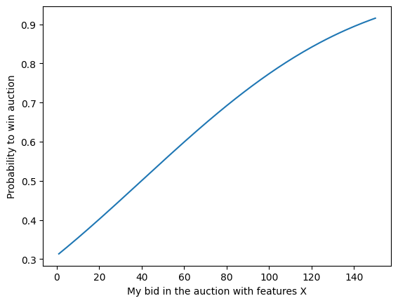
Win rate for the first auction and its input features
data.iloc[0,:]
floor_price     0.00000
partner         2.00000
y              35.10754
Name: 0, dtype: float64
mean,std = pred[0][0], pred[1][0]
mean,std
(39.917053, 79.931786)
Plug the predictions into the CDF and get the winrate for some potential bids
winrate = sp.stats.norm(mean,std).cdf(grid)
plt.plot(grid, winrate)
plt.xlabel("My bid in the auction with features X")
plt.ylabel("Probability to win auction");
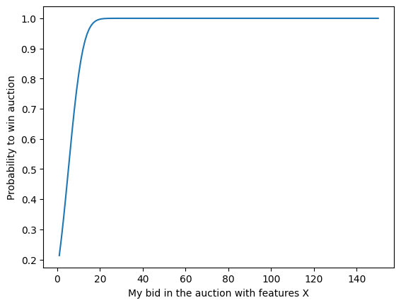
Win rate distribution for the second auction
data.iloc[1,:]
floor_price     2.000000
partner         2.000000
y              89.045763
Name: 1, dtype: float64
mean,std = pred[0][1], pred[1][1]
mean,std
(5.2670693, 5.3625727)
winrate = sp.stats.norm(mean,std).cdf(grid)
plt.plot(grid, winrate)
plt.xlabel("My bid in the auction with features X")
plt.ylabel("Probability to win auction");
Conclusion
Implementing a custom loss function to predict a distribution rather the conditional mean is not difficult. The steps are:
- Pick a suitable distribution.
- Write down the likelihood of the data under the model.
- Simplify it by pulling out constants not needed for minimizing the negative log likelihood.
The tricky part is to think hard and/or check the literature for issues with the estimation approach. For example, the approach I outlined is known to underestimate the variance.
Also, estimation of other moments requires a lot of data. And despite the “big data” I work with, the data available locally, i.e. for each of the combination of feature levels of my input variables can be surprisingly low.
So if you follow this path, don’t ignore what people smarter than me already knew in the 80s and 90s.
Written on March 28th, 2023 by Johannes Haupt