Recalibration after Negative Sampling

This post shows the transformation function that calibrates predictions from a model trained on downsampled data back to the original data. We’ll do the derivation of the transformation and a scikit-learn example with simulated data.

Negative Sampling

Real-time bidding and natural language processing pre-training are two applications were positive cases are much rarer in the data than negative cases. As an example, there are thousands users who don’t click on an ad for each user who does, an even fewer who buy something after the click compared to every user who just ignored it.

When negative cases are so abundant and overall data size is large, it can be helpful to ignore some or even many of the negative cases during model training because they don’t provide much additional information but slow down model estimation because they need to be processed.

A common way to do that is by randomly sampling just a part of the negative cases, while keeping all positive cases in the data. Effectively throwing away negative cases at random decreases the data size, so model estimation generally speeds up. However, by changing the ratio between positive and negative cases, any model estimated on the data (without any correction) will overestimate the probability of positive cases occuring. While we can reasonably expect the model to do distinguish between positive and negative cases equally well (e.g. the AUC doesn’t change), we should expect it to be badly calibrated (e.g. high average probability for positive cases even though they are overall very rare and log-loss decreases on test data which is not sampled).

It is possible to re-calibrate the model predictions to match the original data before resampling. For convenience, I’ll denote the baserate of positive cases $P(y=1)$ in the original data by $b$ and in the re-sampled data by $b’$. The model predictions based on the resampled training data are $p’$, while the predictions that are calibrated for the original data and that we want to use in practice are $p$.

The formulas to know are

1. The rate at which we sample negative cases $w$, which we may empirically optimize or pick to match a particular target ratio of positive vs. negative cases (absent further information often 50:50) \(w = \frac{\text{original ratio}}{\text{target ratio}} = \frac{b}{1-b} \cdot \frac{1-b'}{b'}\)

2. The transformation for the model predictions $p’$ which recalibrates them to calibrated predictions $p$ that match the average occurence rate in the original data \(p = \frac{p'}{p'+\frac{1-p'}{w}}\)

The rest of the post shows how we derive these formulas and what the assumptions are on the way and then shows an example with scikit-learn.

Derivation of the Re-Calibration Formula

A lot of the research around resampling comes from the literature around cost-sensitive learning. Elkan (2001) The Foundations of Cost-Sensitive Learning summarizes the reasoning well and shows many of the, well, foundations in some detail. In that literature, people aim to sample the data to calibrate model predictions so that a 0.5 decision threshold on the probability matches the decision context, made up by the benefits and costs of correct and incorrect decisions. I’ll ignore the cost-informed decision-making background, but their research on resampling data is still helpful and the following derivations are informed by Elkan (2001).

Start with Bayes theorem

Or with our simplified notation

We randomly sample some of the observations for which $y=0$ to create the target, downsampled dataset. Within this dataset, the probability of $y$ given a set of features $x$ changes (there are now more $y=1$ after all, but the distribution of $X$ given $Y$ doesn’t change. Hence $P(y=1|x)$ and $P(y=0|x)$ are different but $P(x|y=1)$ and $P(x|y=0)$ are the same as in the original dataset and we can use this for

We can join these to expression by inserting $\frac{P(x|y=0)}{P(x|y=1)}$ into the expression for $p$. First we reformulate $p’$.

Then we replace $\frac{P(x|y=0)}{P(x|y=1)}$ in the equation for $p$

This is the recalibration formula from above and we see that it works for any downsampling ratio $w$ that we pick. It’s common to downsample to a completely balanced training dataset, i.e. with a target ratio of 1:1, for which $w = \frac{b}{1-b} \frac{0.5}{0.5} = \frac{b}{1-b}$. In practice, less downsampling often gives slightly better models because less data is discarded.

Example

import numpy as np
import matplotlib.pyplot as plt
from sklearn.datasets import make_classification
from sklearn.linear_model import LogisticRegression
from sklearn.metrics import roc_auc_score
from sklearn.calibration import calibration_curve

X, y = make_classification(n_samples=10000, n_informative=10, weights=[0.9])

Here we have some imbalance with a baseline probability for $y$ that is 10%.

y.mean()

0.103

Model without downsampling

logit = LogisticRegression(penalty='none').fit(X,y)

pred = logit.predict_proba(X)[:,1]

pred.mean()

0.10299859038609889

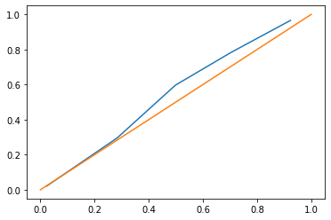
Let’s also have a look at the calibration curve of the predictions to be able to compare later. Logistic regression is usually calibrated well, which is not the case for all machine learning models.

fraction_of_positives, mean_predicted_value = calibration_curve(y, pred, n_bins=5)

np.quantile(pred, [0,0.5, 0.75, 0.9, 0.95, 1])

array([3.78453590e-06, 9.83524180e-03, 4.75441847e-02, 3.33898140e-01,
       8.51368277e-01, 9.99970943e-01])

plt.plot(mean_predicted_value, fraction_of_positives)
plt.plot([0,1],[0,1]);

Model with Downsampling

Downsample the negative cases by a negative sampling rate of 1/9 for a target ratio of 1:1. A ratio of 1:1 is not necessarily the best target ratio in practice, but it is salient because it is “balanced”.

w = 1/9
count_y0 = (y==0).sum()

neg_sample_idx = np.random.default_rng().choice(
    count_y0, size=int(w*count_y0.sum()), 
    replace=False)

neg_sample_idx = np.arange(int(w*(y==0).sum()))

X_sampled = np.vstack([X[y==0][neg_sample_idx], X[y==1]])
y_sampled = np.concatenate([y[y==0][neg_sample_idx], y[y==1]])

X_sampled.shape

(2026, 20)

y_sampled.shape

(2026,)

The new ratio of positive cases is ~50% as expected.

y_sampled.mean()

0.508390918065153

This time we train the model on the downsampled data.

logit = LogisticRegression(penalty='none').fit(X_sampled,y_sampled)

pred = logit.predict_proba(X_sampled)[:,1]

Unsurprisingly, the average prediction is the rate of positive cases in the resampled data, which is much higher than in the original dataset.

pred.mean()

0.5083907547956312

We therefore want to use the formula derived above to re-calibrate the predictions to the original distribution of cases.

def calibrate(p, w):
    return p / (p + ((1-p)/w))

Get the predictions of the model on the original, unsampled dataset.

pred = logit.predict_proba(X)[:,1]

As expected, the model overpredicts the occurance of positive cases.

pred.mean()

0.23492324259220376

pred2 = calibrate(pred,w)

After re-calibration, the average model prediction matches the ratio of positive cases almost exactly.

pred2.mean()

0.09856897573250073

y.mean()

0.103

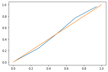
The overall calibration looks also good as judged by the calibration curve of the predictions (close to the diagonal line), at least for the prediction range between 0 and 45% where we find most (95%) of our predictions.

fraction_of_positives, mean_predicted_value = calibration_curve(y, pred2, n_bins=5)

np.quantile(pred2, [0,0.5, 0.75, 0.9, 0.95, 1])

array([1.18645827e-05, 1.07949077e-02, 5.11099944e-02, 3.16203654e-01,
       7.56029748e-01, 9.99710693e-01])

plt.plot(mean_predicted_value, fraction_of_positives)
plt.plot([0,1],[0,1]);