Causal Inference: Contextual Bandit vs. Randomized Trials

Bandit Learning is an approach to causal inference that combines treatment effect estimation and decision making. This post compares the contextual bandit to the conditional mean approach for treatment effect estimation to show that policy learning results in a selection effect that impacts the treatment effect estimate and is difficult to correct ex post.

Making the right decision

import numpy as np
from scipy.stats import linregress
from sklearn.linear_model import LogisticRegression

%matplotlib inline
import matplotlib.pyplot as plt
plt.rcParams["figure.figsize"] = (10,6)
import seaborn as sns

np.random.seed(1234)

Image the following setting: We observe users with a single characteristic $X \sim N(1,1)$. We can choose to not address the user with an action ($t=0$) or can play an action, for example pay to display a banner ad ($t=1$). After we decide on an action, we observe an outcome $y$ that depends on the user characteristic and our action in the following way: \(y =0 + x + t \cdot 2 \cdot x - t \cdot 1+ \epsilon\)

More intuitively: Image we are given the option to display our ad banner to a user and are informed of the user’s estimated age. If the user makes a purchase, we earn a baseline outcome depending on their age plus additional revenue from customer with a higher age if they see the banner, which costs us 1$ to display.

If online marketing is not your thing, image a doctor contemplating medical treatment for a patient. Depending on indicators of the patient’s health, the patient’s expected remaining life is some years plus the benifical effect of treatment, which is higher for healthier patients, and the risks and side effects of the treatment, which on average reduce life expectancy by one year.

def draw_y(x, t):
    return 0 + x + t*2*x -t*1 + np.random.normal(0,1, x.shape[0])

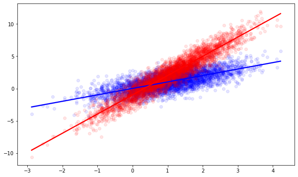
The tradeoff between our actions is of course only known to the Norns, but if we were them we’d observe this situation: For low values of $X$, it’s more profitable to not act, i.e. to refrain from showing a banner or treating the patient. There is a fixed cost of acting. For high $X$, it’s more profitable to act, because the benfits increasingly outweight the fixed cost.

X = np.random.normal(1,1,4000)
sns.regplot(x=X, y=draw_y(X,0),scatter_kws={'alpha':0.1}, color="blue") # Don't act
sns.regplot(x=X, y=draw_y(X,1),scatter_kws={'alpha':0.1}, color="red")  # Act
plt.show()

In many situations our goals are 1. to make the right choice, sit it out or act, when new users come in and 2. to find out the return on the action, which is the factor $2.0 \cdot x$. These goals are clearly related. Once we know the return on the action with high confidence, we can pick the correct action easily. But even before we know the return exactly, we may be able to pick the right action most of the time.

A/B testing: The conditional means approach

Medical research values exact estimation of the return of the action very highly. Randomized Controlled trials, equivalent to A/B testing, are therefore the most common experiment design there. In a nutshell, we randomly choose actions for a while until we are sure of the rewards. Once we are confident enough, we can report what the actual effect of our actions are and should be able to pick the best action.

# Observe a number of users
X = np.random.normal(1,1, size=2000)
# A/B test: Pick one of the two actions randomly for each user
t = np.random.binomial(1,0.5, X.shape[0])
# Observe the reward for each user-action combination
y = draw_y(X, t)

I’ve picked $X$ with a mean of 1, so that the average effect of our actions will be 1. Once we have observed enough users, we should be able to estimate the average effect quite precisely and this average treatment effect is what is reported in most medical, economics or sociology studies.

f"Average Treatment Effect: {y[t==1].mean() - y[t==0].mean()}"

'Average Treatment Effect: 1.1692040412152656'

The average treatment effect indicates that on average, we will be better off giving every person the treatment than giving nobody the treatment.

In our setting, the effect of our action varies with the user characteristic, which is called a heterogeneous treatment effect. One way to estimate the effect of our action conditional on the user characteristic is to look at the difference between two models, one predicting the reward under treatment and one predicting the reward without treatment.

This and most other approaches rely on a few assumptions, in particular that the treatment was assigned to users randomly so that each user had a chance to receive the treatment. This assumption is neatly fulfilled by our randomized A/B test.

It’s worth pointing out that the purpose of randomization is not to choose the action in the experiment with equal chance, although that increases statistical confidence in the estimate. The purpose is to give every person the same chance to be treatment during the experiment, indepedent of their characteristic $X$.

f"Sample sizes: {(X[t==1].shape[0], X[t==0].shape[0])}"

'Sample sizes: (993, 1007)'

# Predicting the outcome from users who got the treatment
beta_T,_,_,_,_ = linregress(X[t==1], y[t==1])

f"Payoff estimate Treatment: {beta_T}"

'Payoff estimate Treatment: 3.0437511490333207'

# Predicting the outcome from users without treatment
beta_C,_,_,_,_ = linregress(X[t==0], y[t==0])

f"Payoff estimate Control: {beta_C}"

'Payoff estimate Control: 1.0075894921383526'

# The difference in predictions is the treatment effect
f"Treatment effect coefficient: {beta_T - beta_C} (True: 2.0)"

'Treatment effect coefficient: 2.036161656894968 (True: 2.0)'

This worked nicely to tell us the actual treatment effect in relation to the characteristic with a bit of uncertainty! We could check its statistical significance, too, to be confident in our estimate. Since we know the treatment effect given any value of $X$ now, we can now easily decide which action to take.

Of course, this knowledge came at a cost: we had to randomly treat 4000 users to build our models. Why was that necessary? To observe what would happen to users with different characteristic with and without the treatment.

We can see this nicely by looking at the distribution of the user characteristic in both groups, with and without the action.

sns.kdeplot(X, color='grey') # Overall characteristics
sns.kdeplot(X[t==1], color="blue") # Found in the treatment group
sns.kdeplot(X[t==0], color="red")  # Found in the control group
plt.show()

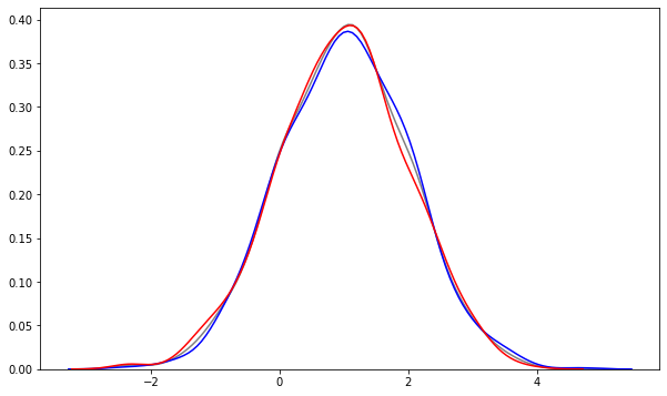
In both groups we have observed users with characteristics that are almost exactly the same and match the overall distribution of the characteristic.

LinUCB

Reinforcement Learning, Bandit Learning or Policy Learning shift the focus from getting the most accurate estimate of the treatment effect to making good choices while improving our estimate. Their focus lies on finding the better action as quickly as possible, even if that means that we might be less certain about the actual outcome of the action. The idea is that the exact value is not needed for good decision making as long as we are confident that the action is better than any other action. The purpose of policy learning is to ultimately settle on the best decision policy, but make as few bad decisions as possible before settling.

The recent Covid pandemic is a sad example where doctors have to make informed decisions based on their current knowledge at the same time as collecting data to inform future decisions.

One popular bandit learning algorithm is the linear upper confidence bound bandit (linUCB). In short, it works by making a rough guess about how good the outcome of an action might be, the upper confidence bound. Actions may look good if they have a high certain reward and/or if we are still uncertain about the reward. The linUCB bandit always picks the action with the highest expected reward plus its upper confidence bound.

John Langford is a big name associated with these algorithms, but I’d recommend this paper for a summary: Dimakopoulou, M., Zhou, Z., Athey, S., & Imbens, G. (2018). Estimation Considerations in Contextual Bandits. ArXiv:1711.07077 [Cs, Econ, Stat]. http://arxiv.org/abs/1711.07077

Or follow the steps of the lazy implementation below:

# Calculate the upper confidence bound
def calc_ucb(x, X):
    x = np.array(x, ndmin=2)
    X = np.array(X, ndmin=2)
    # xt (XtX)^-1 x
    return np.dot(x.transpose(), np.linalg.inv(np.dot(X.transpose(), X))).dot(x)

# Logging setup
x_log = []
y_log = []
t_log = []
p_log = []

beta_T_log = []
beta_C_log = []

ucb_T_log = []
ucb_C_log = []

beta_T = 1
beta_C = 1

X_T = np.array([10], ndmin=2)
X_C = np.array([10], ndmin=2)

y_T = np.array([10], ndmin=2)
y_C = np.array([10], ndmin=2)

# Exploration factor
# We increase or decrease the confidence bound 
# to encourage or discourage exploration of the actions
alpha=1.

# Experiment loop
for i in range(2000):
    # Look at one next user
    x = np.random.normal(1,1,[1,1])
    
    # Cold-start using random treatment allocation
    # For the first rounds we play randomly until we get a feeling 
    # for the outcomes and our certainty about them
    if i<20:
        a = np.random.binomial(1,0.5,1)
        if a==1:
            y_temp=draw_y(x,1) # Observe outcome
            y_T = np.r_[y_T, y_temp] # Add outcome to list
            X_T = np.r_[X_T, x] # Add user to list
            beta_T, c_T,_,_,_ = linregress(X_T.flatten(), y_T.flatten()) # Update regression
        else:
            y_temp=draw_y(x,0)
            y_C= np.r_[y_C, y_temp]
            X_C = np.r_[X_C, x]
            beta_C ,c_C,_,_,_ = linregress(X_C.flatten(), y_C.flatten())
        
        # Log probability for the action
        p_log.append(np.array([0.5]))
        ucb_T_log.append(np.array([0.]))
        ucb_C_log.append(np.array([0.]))
        
        
    ### <--- Real linUCB Bandit starts here ---> ###    
    # Decide whether to play treatment based on UCB    
    else:
        # Calculate UCB
        ucb_T = alpha * np.sqrt( calc_ucb(x, X_T) )
        ucb_C = alpha * np.sqrt( calc_ucb(x, X_C) )
        
        # Pick higher estimate + UCB for treatment
        a = 1*(
            (c_T + beta_T*x + ucb_T) >= (c_C + beta_C*x + ucb_C)
        ).flatten()
        
        # Log results
        if a==1:
            # Add observation and observed outcome data
            y_temp=draw_y(x,1)
            y_T = np.r_[y_T, y_temp]
            X_T = np.r_[X_T, x]
            # Estimate model using the added data
            # Could improve scalability using online learning
            beta_T,c_T,_,_,_ = linregress(X_T.flatten(), y_T.flatten())
            
        elif a==0:
            y_temp=draw_y(x,0)
            y_C= np.r_[y_C, y_temp]
            X_C = np.r_[X_C, x]
            beta_C ,c_C,_,_,_ = linregress(X_C.flatten(), y_C.flatten())
            
        else:
            print("Error")
            
        # Log probability of this action at time of decision
        propensity_model = LogisticRegression(penalty="none")
        propensity_model.fit(np.array(x_log).reshape(-1,1), np.array(t_log))
        if a==1: 
            p = propensity_model.predict_proba(x)[:,1] # Chance of being in treatment group
        else:
            p = propensity_model.predict_proba(x)[:,0] # Chance of being in control group
        p_log.append(p)
        
        # Log UCB
        ucb_T_log.append(ucb_T)
        ucb_C_log.append(ucb_C)

    # Logging
    y_log.append(y_temp)
    x_log.append(float(x))
    t_log.append(int(a))
            
    beta_T_log.append(beta_T)
    beta_C_log.append(beta_C)
        
    

# Cleanup
y_log = np.array(y_log).flatten()
p_log = np.array(p_log).flatten()
t_log = np.array(t_log).flatten()

X_T, X_C = X_T[1:,:], X_C[1:,:]
y_T, y_C = y_T[1:], y_C[1:]

The bandit is more selective when trying out the actions. Because it estimates quickly that the treatment is, on average, the better choice, it chooses the treatment action about 2/3 of the time.

f"Sample sizes (Treatment, Control): {(X_T.shape[0], X_C.shape[0])}"

'Sample sizes (Treatment, Control): (1539, 461)'

Since we pick the control action less often than in the A/B test, our estimate of the treatment effect is less accurate. It is accurate enough to determine that the treatment is better than doing nothing, but we are less certain of how much better exactly.

f"Coefficient X Treatment: {beta_T}"

'Coefficient X Treatment: 2.7493601815739885'

f"Coefficient X Control: {beta_C}"

'Coefficient X Control: 1.0409441555900563'

# Estimate the treatment effect as before
f"Treatment effect coefficient: {beta_T - beta_C} (True: 2.0)"

'Treatment effect coefficient: 1.7084160259839323 (True: 2.0)'

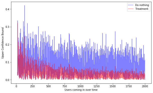
We can see the focus on the treatment group by looking at the upper confidence bound over time, which measures our uncertainty about the outcome. The uncertainty in the treatment group decreases much quicker than in the control group, because we play the action more often.

y_T_log = (np.array(x_log)*np.array(beta_T_log)).flatten()
y_C_log = (np.array(x_log)*np.array(beta_C_log)).flatten()

y_T_ucb_log = y_T_log + np.array(ucb_T_log).flatten()

y_C_ucb_log = y_C_log + np.array(ucb_C_log).flatten()

warmup = 20
plt.plot(np.arange(warmup,len(ucb_C_log)),np.array(ucb_C_log).flatten()[warmup:], alpha=0.5, color="blue")
plt.plot(np.arange(warmup,len(ucb_T_log)),np.array(ucb_T_log).flatten()[warmup:], alpha=0.5, color="red")
plt.legend(["Do nothing","Treatment"])
plt.xlabel("Users coming in over time")
plt.ylabel("Upper Confidence Bound")
plt.show()

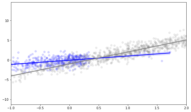
The uncertainty is generally higher in the no-action group but we are more uncertain about some users than about others. Compare the 95%-confidence intervals for the regression on the control group (blue) against the regression on the control group from the A/B test. In the area to the right where we don’t observe users, the uncertainty about the treatment effect is naturally larger.

fig, ax = plt.subplots()
ax.set_xlim(-1,2)
#sns.regplot(x=X_T, y=y_T,scatter_kws={'alpha':0.1}, color="blue") # Don't act
sns.regplot(x=X_C, y=y_C, ci=99, scatter_kws={'alpha':0.15}, color="blue", ax=ax)  # Act
sns.regplot(x=X[t==1], y=y[t==1], ci=99,scatter_kws={'alpha':0.15}, color="grey", ax=ax)  # Act
plt.show()

But that is not all. The characteristics of users that we observe in the control group are now completely different from the users in the treatment group. When we get into higher $x$ values, then the expected return in the treatment group is clearly higher and the control group gets explored less often. Conversely, for low x values, the bandit explores the treatment less often because the treatment is clearly not working here. When using this data as training data or for treatment effect estimation, the different distribution of x in the groups causes a selection bias. We violate the assumption that every user has some chance to see each action (user with X=4 are always treated) and the characteristics in each group are very different from the overall distribution of $X$.

sns.kdeplot(x_log, color='grey')
sns.kdeplot(X_T.flatten(), color='blue')
sns.kdeplot(X_C.flatten(), color='red')
plt.show()

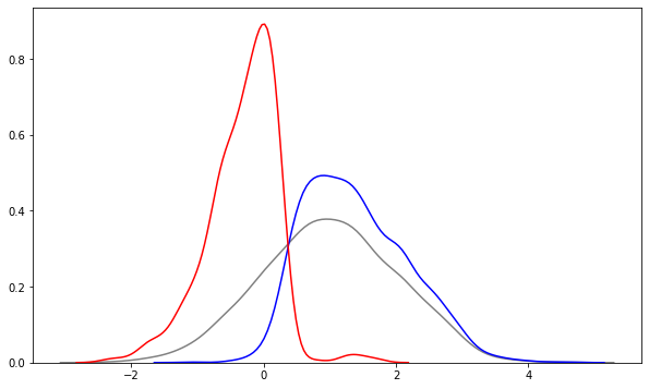
There are well-understood methods to correct for this imbalance between the groups, e.g. matching observations based on their characteristics or inverse propensity weighting. These work well for areas where we observe too few or too many of a group, like between 0 and 1. They don’t work where we don’t observe any user in a group, like treated users below an $X$ of 0 or untreated users above an $X$ of 2. For these users, we just don’t have any information and can at best extrapolate from the observed cases.

Conclusion

A/B testing and bandit learning are approaching the same problem: Which of several actions leads to the best outcome? We have seen that A/B testing explores the outcomes for different users randomly to estimate the outcome of each action accuractly after exploration. Bandit learning minimizes the number of bad decisions while exploring, but leads to sample selection issues that in turn lead to less accurate estimates of the outcomes of each action.