Johannes Haupt remerge.io
Accelerated Bayesian Causal Forest (XBCF)
This post shows how to use Accelerated Bayesian Causal Forest (XBCF) to estimate the conditional average treatment effect (or uplift) using a specialized version of Bayesian Additive Regression Trees (BART). It’s better described as Bayesian boosted trees for non-parametric causal inference.
The Python version of the package is available here: https://github.com/socket778/XBCF and can be installed with pip install xbcausalforest. I’m indebted to Nikolay Krantsevich who develops and maintains the package and answered additional questions I had. The model is introduced in Hahn et al. (2017)’s Bayesian Regression Tree Models for Causal Inference and I hear there will be a paper expanding on the results there in the near future.
import numpy as np
import pandas as pd
import matplotlib.pyplot as plt
import seaborn as sns
from xbcausalforest import XBCF
Simulating Data
I’ll simulate data from a randomized experiment. The treatment effect differs between subjects and depends on some observed covariates $X$. Intuitively, imagine that the effect of some medication depends on the age and weight of the patient or that the additional spend due to a coupon depends on the value of the shopping basket and the time on product pages so far.
Because the difference is large enough to change our decision whether to apply the treatment, we want to know not only the average effect for any subject, but the more precise effect of the treatment on a single subject given what we know about her.
We would have a number of people N and for simplicity, let’s say we have only k=2 variables that influence the observed outcome y and the effect $\tau$ of the treatment. The data is the result of a randomized trial with a 50:50 split and we have encoded the treatment group as z=1 and the comparison group as z=0.
# number of observations N and number of covariates k
N = 20000
k = 2
p_T =0.5
The data follows the following data generating process:
- $z\sim Binomial(p=0.5)$
- $\tau = 2 + 0.5X_2 + 0.5X_2^2 - 0.5X_1^2 - 3\cdot\mathbf{I}(X_1>0)$
- $y \sim \mathcal{N}(\mu=100 + 5X_1 - 5X_2 + 2X_1^2 + 5X_1X_2 + z\tau, \sigma=2)$
# Simulate data
def data_generating_process(X):
    z = np.random.binomial(1, p_T, size=(N,))
    effect = 2 + 0.5*X[:,1] + 0.5*X[:,1]**2 - 0.5*X[:,0]**2 - 3*(X[:,0]>0)
    mu = 100 + 5*X[:,0] - 5*X[:,1] + 2*X[:,0]**2 + 5*X[:,0]*X[:,1]
    y = np.random.normal(mu, scale=2, size=(N,)) + z*effect
    return y, z, effect

X      = np.random.multivariate_normal([0,0], np.array([[1,0.1],[0.1,1]]), size=(N,))
X_test = np.random.multivariate_normal([0,0], np.array([[1,0.1],[0.1,1]]), size=(N,))

y, z, effect      = data_generating_process(X)
_, _, effect_test = data_generating_process(X_test)
y[z==0].mean(), y[z==0].std()
(102.57304278398883, 9.436481265966025)
effect.mean(), effect.std()
(0.4904417000455662, 1.848151821851121)
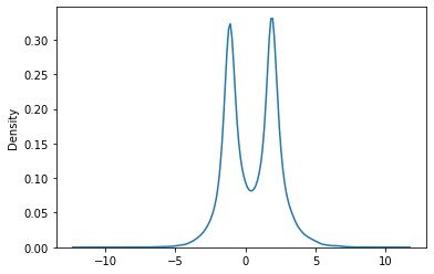
This is what the range of treatment effects looks like: it’s mostly between -5 and 5 but with two peaks in the middle. The effect depends on the observed covariates in a nonlinear way.
Note that in this setting where the distribution of the effect has more than one peak, it’s useful to predict the treatment effect for an individual because the average treatment effect of 0.5 doesn’t describe the effect on a particular individual very well. This treatment actually has a negative effect on some people and a positive effect on others.
effect.min(), effect.mean(), effect.max()
(-11.549275452228715, 0.4904417000455662, 10.959946990413645)
import seaborn as sns
sns.kdeplot(effect);
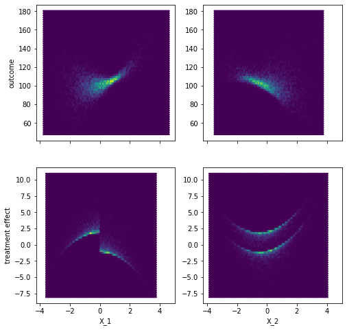
fig, axes = plt.subplots(2,2, sharey=False, sharex=True, figsize=(8,8))
# Relation X to y
axes[0,0].hexbin(X[z==0,0], y[z==0],)
axes[0,1].hexbin(X[z==0,1], y[z==0],)
# Relation X to treatment effect
axes[1,0].hexbin(X[z==1,0], effect[z==1])
axes[1,1].hexbin(X[z==1,1], effect[z==1])

axes[0,0].set_ylabel("outcome")
axes[1,0].set_ylabel("treatment effect")
axes[1,0].set_xlabel("X_1")
axes[1,1].set_xlabel("X_2")
Accelerated Bayesian Causal Forest
The parameters include those that are set for the Bayesian Tree Ensemble and those specific to the specification to estimate the heterogeneous treatment effect.
An important insight is that the specifcation of the causal model is a sum of two parts: \(E[Y=y_i |X=x_i,Z=z_i] = \mu(x_i) + \tau(x_i)z_i\)
The first part $\mu(x_i)$ is a BART model to estimate the expected outcome from a set of covariates and, if required, an estimate of the probability to receive treatment. The parameters for this BART model are denoted with pr for ‘prognostic’, e.g. num_trees_pr.
The second part $\tau(x_i)$ is a BART model that estimates the treatment effect conditional on some covariates, with its parameters denoted by trt as in ‘treatment’.
Since the two parts are separate models, there is flexibility in their specification. First, the same or a different set of covariates can be passed to the two models. If it is plausible that the outcome and treatment effect depend on different covariates, only those covariates can be passed to each BART. Second, the parameters passed to each model can be different. The BART for the treatment effect may be a bit smaller/more restricted, because it may be plausible that the outcome depends on the covariates in a more complex way than the treatment effect, especially when we are used to assume a constant treatment effect for all individuals.
The BART models are not estimated by standard MCMC, but the XBART (Accelerated BART) algorithm. The Parameters that control the BART estimation are:
num_cutpoints: Number of cutpoints that are tested as splits for continuous covariatesnum_sweeps(andburnin): Number of MCMC draws (and the number of MCMC draws that is discarded as warm up/burn-in).
Parameters that control the size of the BART ensemble:
num_trees: Number of trees in the ensemble. Somewhere between 10 and a few hundred.Nmin: Minimum number of samples in the final leavesalpha,beta: Control the tree depth by setting a prior for the probability that the current leaf is a final leaf formalized by $p(\text{leaf at depth t is not final leaf}) = \alpha(1+d)^{-\beta}$. A loweralphaand higherbetamake the trees more shallow. Chipman et al. (2010) suggest $\alpha=0.95, \beta=2$.alphaseems reasonable between [0.5,0.95] andbetabetween [1, 2].mtry: Number of variables to try at each split. From my experience with gradient boosted trees, I prefer closer to all of them.tau: Prior on the variance in the leaf for each tree. Hahn et al. propose to scale the prior with some factor of the variance of the outcome divided by the number of trees. Intuitively, this is our prior understanding of how much variation in the observed outcome is due to other factors and how much is due to the treatment.
Of these, the prior for the precision in the leaves, tau, has been the most important for me to set correctly to get reasonable results. The explanation in Hahn et al. (2020) Section 5.2 was too brief for me to fully understand, so I recommend a look into the original Chipman et al. (2010) paper on BART, specifically Section 2.2.3.
tau_pr = 0.6*var(y)/num_trees_pr and tau_trt=0.1*var(y)/num_trees_trt are suggested defaults, attributing 60% of the variation to the non-treatment part in the model, 10% to the treatment part and the rest to noise. I consider 10% due to treatment too optimistic, but I haven’t explored the sensitivity of the model to this prior in detail.
NUM_TREES_PR  = 200
NUM_TREES_TRT = 100

cf = XBCF(
    #model="Normal",
    parallel=True,
    num_sweeps=50,
    burnin=15,
    max_depth=250,
    num_trees_pr=NUM_TREES_PR,
    num_trees_trt=NUM_TREES_TRT,
    num_cutpoints=100,
    Nmin=1,
    #mtry_pr=X1.shape[1], # default 0 seems to be 'all'
    #mtry_trt=X.shape[1],
    tau_pr = 0.6 * np.var(y)/NUM_TREES_PR, #0.6 * np.var(y) / /NUM_TREES_PR,
    tau_trt = 0.1 * np.var(y)/NUM_TREES_TRT, #0.1 * np.var(y) / /NUM_TREES_TRT,
    alpha_pr= 0.95, # shrinkage (splitting probability)
    beta_pr= 2, # shrinkage (tree depth)
    alpha_trt= 0.95, # shrinkage for treatment part
    beta_trt= 2,
    p_categorical_pr = 0,
    p_categorical_trt = 0,
    standardize_target=True, # standardize y and unstandardize for prediction
         )
Since we specify the model as a sum of two BARTs, we can pass different sets of covariates to the outcome model and the treatment model, denoted by x and x_t. z is the treatment indicator coded 0/1.
There might still be an unfixed issue causing the fit function to crash when the treatment indicator is defined as a float. To be safe, I change the type of the treatment indicator to int.
z= z.astype('int32')
Note that for a dataset of 20k observations and MCMC estimation, training and prediction are still very fast.
%%time
cf.fit(
    x_t=X, # Covariates treatment effect
    x=X, # Covariates outcome (including propensity score)
    y=y,  # Outcome
    z=z, # Treatment group
)
CPU times: user 24.6 s, sys: 932 ms, total: 25.5 s
Wall time: 18.8 s

XBCF(num_sweeps = 50, burnin = 15, max_depth = 250, Nmin = 1, num_cutpoints = 100, no_split_penality = 4.605170185988092, mtry_pr = 2, mtry_trt = 2, p_categorical_pr = 0, p_categorical_trt = 0, num_trees_pr = 200, alpha_pr = 0.95, beta_pr = 2.0, tau_pr = 0.23585769147754146, kap_pr = 16.0, s_pr = 4.0, pr_scale = False, num_trees_trt = 100, alpha_trt = 0.95, beta_trt = 2.0, tau_trt = 0.07861923049251382, kap_trt = 16.0, s_trt = 4.0, trt_scale = False, verbose = False, parallel = True, set_random_seed = False, random_seed = 0, sample_weights_flag = True, a_scaling = True, b_scaling = True)
Predictions for out-of-sample data and model evaluation
The predict method can be used to get num_sweeps posterior samples for a new or out-of-sample set of observations with covariates x.
%%time
tau_xbcf = cf.predict(X_test, return_mean=True)
CPU times: user 1 s, sys: 11.3 ms, total: 1.01 s
Wall time: 1.01 s
Note that the predict function does the rescaling of the treatment effect estimate by the “estimated coding of Z” saved in cf['b'] discusssed in Section 5.3 of Hahn et al. (2020).
In real appliations, we naturally don’t know the true effect, but since we simulated the data here, we can compare the predictions to the true effect.
# Average treatment effect calibration
np.mean(effect_test), np.mean(tau_xbcf)
(0.5098960761277523, 0.5053294157578107)
# Poor man's calibration plot
plt.figure(figsize=[4,4])
plt.xlim([-10,10])
plt.ylim([-10,10])
plt.scatter(effect_test, tau_xbcf, alpha=0.5)
plt.xlabel('True effect')
plt.ylabel('XBCF prediction');
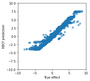
The predictions look surprisingly good to me. We can see that the model is not well calibrated towards the extremes, where it underestimates the true treatment effect, but for most observations it predicts the treatment effect with what looks like less than plus/minus 2.
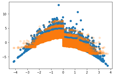
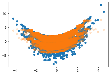
Looking into the relation between the covariates and the model prediction, we see that the model finds the step at $X_1>0$ and nicely approximates the quadratic shapes. I’d guess that we could approximate the extremes even better with more trees or less regularization.
plt.scatter(X_test[:,0], effect_test)
plt.scatter(X_test[:,0], tau_xbcf, alpha=0.2)
<matplotlib.collections.PathCollection at 0x7f907f662e10>
plt.scatter(X_test[:,1], effect_test)
plt.scatter(X_test[:,1], tau_xbcf, alpha=0.2)
<matplotlib.collections.PathCollection at 0x7f906ab41bd0>
It’s worth mentioning that we can use the posterior draws from the XBCF to generate credible intervals for individual predictions easily, although we should probably draw more samples for better accuracy.
tau_posterior = cf.predict(X_test, return_mean=False)[:,cf.getParams()['burnin']:]
tau_posterior.shape
(20000, 35)
These are the 95% credible intervals for the first five observations based on the quantiles of the posterior predictive.
pd.DataFrame(np.quantile(tau_posterior[:5], [0.05,0.95], axis=1).T, columns=['CI lower', 'CI upper'])
| CI lower | CI upper | |
|---|---|---|
| 0 | 1.610548 | 2.188137 |
| 1 | 2.943488 | 3.508837 |
| 2 | 1.348259 | 1.980816 |
| 3 | 5.016946 | 6.014521 |
| 4 | 1.725381 | 2.247120 |
Benchmarks
We can compare that to other non-parametric approaches to estimate the conditional average treatment effect.
Two-Model Approach
Let’s use a simple approach first: Train two models, one for each experiment group. The test group model tells us the outcome if we apply treatment, the control group model predicts the outcome if we don’t apply treatment. The difference between the two is the treatment effect.
from sklearn.ensemble import RandomForestRegressor

reg1 = RandomForestRegressor(max_samples=0.8, bootstrap=True, min_samples_leaf=50).fit(X[z==1,:],y[z==1])
reg0 = RandomForestRegressor(max_samples=0.8, bootstrap=True, min_samples_leaf=50).fit(X[z==0,:],y[z==0])

tau_tm = reg1.predict(X_test) - reg0.predict(X_test)
plt.figure(figsize=(4,4))
plt.xlim([-10,10])
plt.ylim([-10,10])
plt.scatter(effect_test, tau_tm, alpha=0.4);
plt.xlabel('True effect')
plt.ylabel('Two-Model prediction');
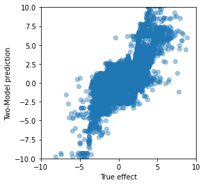
Not terrible for such a simple approach. The range looks alright and we can see the positive linear relationship between the actual and predicted treatment effect, although the individual predictions can be so far off that observations with a clearly positive reaction are estimated to be negative and vice versa.
Double-Robust Estimation
A more advanced but technically easy approach is to use double-robust estimation and train a model to predict a transformed outcome. We know the treatment for the training data was assigned randomly with probability 0.5, so I won’t train a propensity model, but we still need to train to outcome models for the transformation.
# Outcome models
mu0_rf = RandomForestRegressor(max_samples=0.8, bootstrap=True, min_samples_leaf=50).fit(X[z==0,:], y[z==0])
mu1_rf = RandomForestRegressor(max_samples=0.8, bootstrap=True, min_samples_leaf=50).fit(X[z==1,:], y[z==1])
The formula for the double-robust outcome transformation:
# Double-robust outcome transformation
y_dr = mu1_rf.predict(X) - mu0_rf.predict(X) +\
        (z*    (y-mu1_rf.predict(X))/p_T) - ((1-z)*(y-mu0_rf.predict(X))/p_T)
And finally training a model on the transformed outcome:
# Treatment effect model
rf_dr = RandomForestRegressor(n_estimators=300, max_depth=10, min_samples_leaf=50,
                              max_samples=0.8, bootstrap=True).fit(X, y_dr)
tau_dr = rf_dr.predict(X_test)
plt.figure(figsize=(4,4))
plt.xlim([-10,10])
plt.ylim([-10,10])
plt.scatter(effect_test, tau_dr)
plt.xlabel('True effect')
plt.ylabel('Double-robust prediction');
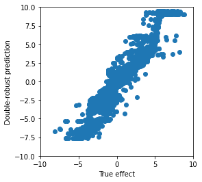
These predictions are clearly better than the two-model approach, but even with some manual parameter tuning they are are worse than the XBCF predictions. Naturally, this is just a small toy example, but it matches the good performance that I’ve seen in a real-world application.
To be sure, we can look at the mean squared error between the predictions of each model and the true effect.
# XBCF
np.mean((effect_test - tau_xbcf)**2)
0.07067651668001747
# Two-Model
np.mean((effect_test - tau_tm)**2)
1.3625449080780299
# Double-Robust
np.mean((effect_test - tau_dr)**2)
0.3354657645875019
Conclusion
I find the decomposition of the outcome into a “prognostic term” and a “treatment term” exceedingly interesting and have seen it before in Farrell et al. (2018’s Deep Neural Networks for Estimation and Inference. Specifying the model with two BART priors is a great way to have Bayesian model with, for example, easy credible intervals while also relying on a non-parametric estimation to capture complex effect heterogeneity. The Accelerated Bayesian Causal Forest (XBCF) seems to be an excellent CATE model and sufficiently scalable for marketing data of reasonable size.
Written on March 28th, 2021 by Johannes Haupt